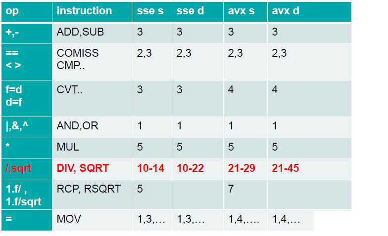
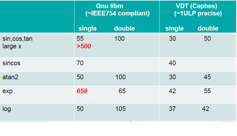
Cost of Operations

when we discuss numerical computation, you will see the non-integer numbers referred as floating point numbers.
numbers is a computer a represented with a finite numbers of bits. integers are simply the traditional integer numbers expressed in binary format, and can range from 8 bits (one byte) to 64 bits
How would you represent a number with a non integer part?
one could use a fixed part of your available bites to represent the integer part and another one to represent the floating point part, but this would severely limit the range of numbers that can be described.
the other option is to use the scientic notation to represent them: this way you can get almost as big or small as needed!
To represent the number we divide it in 3 components:
so the number will represent the following:
$n = (-1)^s \cdot S \cdot 2^e$
due to the limited nature of the floating point numbers, we will have problems representing some numbers:
the first one might not be a surprise, but the second one is quite surprising: the information contained in them is finite!
the problem is that those numbers still requires an infinite number of digits to be written down.
think of the fraction $2/3 = 0.(\overline{6})$
if one has to work with a finite number of digits, it would be represented as: $2/3 = 0.66666667$
that is an approximation, and could lead to numerical imprecision, but it's the best we can do with finite space.
A common source of errors is that the "simple" fractions in base ten might not have a finite representation in base 2.
for example, 0.1, is represented as $0.0(\overline{0011})$
# writing 0.1 with 32 significant digits
print("{:f} = {:.32f}".format(0.1, 0.1))
print("{:.17f} + {:.17f} = {:.17f}".format(0.1, 0.2, 0.1 + 0.2))

# python hides the horrible truth from you
print(0.1)
0.100000 = 0.10000000000000000555111512312578
0.10000000000000001 + 0.20000000000000001 = 0.30000000000000004
0.1
therefore:
0.1 + 0.1 + 0.1 - 0.3
returns
$5.5\ldots \cdot 10^{-17}$
instead of 0
Python works with 53 bit of precision, so the values that is working with internally are not the same as the ones that it shows using a simple print
"If Python were to print the true decimal value of the binary approximation stored for 0.1, it would have to display 0.1000000000000000055511151231257827021181583404541015625 that is more digits than most people find useful."
Due to their structure, floating point arithmetics is not equivalent to the one you are familiar with using the real numbers
a = 0.1
b = 0.2
c = 0.3
print((a + b) + c, a + (b + c))
#verify the associative property (+) including all bits
assert((a + b) + c == a + (b + c))
0.6000000000000001 0.6
---------------------------------------------------------------------------
AssertionError                            Traceback (most recent call last)
<ipython-input-4-1b280911bc05> in <module>
      3 c = 0.3
      4 print ((a + b) + c, a + (b + c))
----> 5 assert((a + b) + c == a + (b + c)) #verifica della proprietà associativa(+) considerando tutti i bit

AssertionError:
Exact fractions, on the other end, are all the fractions that can be expressed as $1/2^N$:
for an extensive explaination, read What Every Computer Scientist Should Know About Floating-Point Arithmetic
if you have to test is two floating point numbers are close enough to be for all intent and purposes considered equal, you can use the function math.isclose:
>>> import math
>>> a = 5.0
>>> b = 4.99998
>>> math.isclose(a, b, abs_tol=0.00003)
True
>>> math.isclose(a, b, abs_tol=0.00001)
False
>>> math.isclose(a, b, rel_tol=1e-5)
True
>>> math.isclose(a, b, rel_tol=1e-6)
False
If you don't care about numerical performances, you can also use the builtins modules decimal and fraction
>>> from decimal import getcontext, Decimal
>>> getcontext().prec = 6
>>> Decimal(1) / Decimal(7)
Decimal('0.142857')
>>> getcontext().prec = 28
>>> Decimal(1) / Decimal(7)
Decimal('0.1428571428571428571428571429')
>>> from fractions import Fraction
>>> Fraction(16, -10)
Fraction(-8, 5)
>>> Fraction('-3/7')
Fraction(-3, 7)
>>> Fraction('1.414213')
Fraction(1414213, 1000000)
>>> Fraction('7e-6')
Fraction(7, 1000000)
>>> Fraction(2.25)
Fraction(9, 4)
>>> Fraction(1.1) # why?
Fraction(2476979795053773, 2251799813685248)
>>> from decimal import Decimal
>>> Fraction(Decimal('1.1'))
Fraction(11, 10)
alongside precision errors and round offs, there are several possible exceptions that can be raised while operating with floating point numbers.
They are defined by the IEEE standard
Underflow : the result of an operation is too small to be represented with a number
Overflow : the result of an operation is too big to be represented with a number
Divide-by-zero : when one tries to divide by 0
Invalid : when the operation is not well defined (es. (0.0 / 0.0).
Inexact : happens when the result of the operation is strongly approximated
Given the properties of the floating point numbers, different ways of performing your calculations can yield wildly different results!
choosing the best algorithm is a craft, that needs to consider the floating point arithmetics, but also to balance it with the computational requirements in terms of memory and time!
Lets suppose that we want to evaluate the average of a vector $x$.
we can estimate it using
$E[x] = \sum_{i=1}^N \frac{x_i}{N}$
or
$E[x] = \frac{1}{N}\sum_{i=1}^N x_i$
From a real number perspective these two versions are exactly equal, but for floating points they are not!
import random
N = 1000
x = [random.normalvariate(mu=0, sigma=0.1) for i in range(N)]
mean_1 = 0.0
mean_2 = 0.0
for x_i in x:
    mean_1 += x_i / N
    mean_2 += x_i
mean_2 /= N
print("Media 1 = {:.32g}".format(mean_1))
print("Media 2 = {:.32g}".format(mean_2))
print("difference = {:.4g}".format(mean_2-mean_1))
Media 1 = -0.001613657043592960516759093891892
Media 2 = -0.0016136570435929592157164869092867
difference = 1.301e-18
For the estimate of the variance the results can be even more extremes:
in certain cases we can obtain a negative variance using the usual formula!
if you want to read more, check Comparing three methods of computing standard deviation
On the other end, sometimes a less precise algorithm can be preferred simply due to its speed.
On a traditional CPU different operations have wildly different execution times, and this could lead to dramatic differences in approach!

A consequence of this is that performing different operations that should be the same can have massive performance gain. (an example with a spoiler)
import numpy as np
a = np.random.randn(100_000)
%timeit a/2
59.4 µs ± 1.42 µs per loop (mean ± std. dev. of 7 runs, 10,000 loops each)
%timeit a*0.5
35.6 µs ± 632 ns per loop (mean ± std. dev. of 7 runs, 10,000 loops each)
this can create some mind bending effect performance wise
%timeit a*1/2
101 µs ± 1.74 µs per loop (mean ± std. dev. of 7 runs, 10,000 loops each)
%timeit 1/2*a
37.1 µs ± 336 ns per loop (mean ± std. dev. of 7 runs, 10,000 loops each)
A classic example from computer science is the inverse of a square root of a number
$$ \frac{1}{\sqrt{x}} $$you could use the standard formula, and obtain a reasonably good result:
from math import sqrt
print(1/sqrt(4))
0.5
somebody (it is actually not known who) developed the following monster to do the same operation
def isqrt(number):
    import numpy as np
    assert number > 0
    threehalfs = 1.5
    x2 = number * 0.5
    y = np.float32(number) # converting the number to float32

    i = y.view(np.int32) #convert y to a int32 variable
    magic = np.int32(0x5f3759df) # magic number,  nobody knows why it works
    i = magic - np.int32(i >> 1) #difference bit-wise of the numbers
    y = i.view(np.float32)

    y = y * (threehalfs - (x2 * y * y))
    return float(y)

print(isqrt(4))
0.49915357479239103
This algorithm is less precise and more complicated, but it's so much faster than the naive implementation that is single handedly considered the code that allowed the birth of modern first person shooting games!
this is because this expression appears countless times in the dynamic light computation (to decrease it with distance), and this was fast and precise enough to allow to be used in real time
note: this algorithm is actually performing the first step of a newton minimization algorithm

there are several ways to speed up and optimize an algorithm, and each one of them is appropriate to different situations:
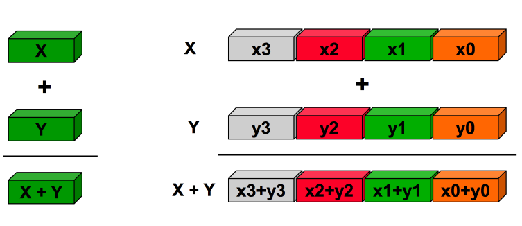
The last one is the idea of expressing operations on entire data structures, and letting the CPU perform them on all the element at once.
the performance increase comes from a reduction of the cache I/O between CPU and RAM, a huge bottleneck in operations. (we will see the numexpr library for even more optimization)

So we can use vectorization when:
vectorization is one of the easiest methods to implement and that have the best gain for effort... especially in high level programming languages
Numpy is the library that underpins all the python scientific ecosystem, for high performance computation and data analysis
The library provides an object, the array (ndarray, to be specific), that support vectorized and parallel computation, allowing high performance math in python, to a speed that can rival C (if properly implemented)
The library also provides most common manipulation algorithms (later we'll discuss the extensions with scipy), all implemented in a vectorized fashion, but also read and write capabilities, tabular data manipulation, linear algebra, and even C++ code wrapping!
Good reference book (free online) are:
import numpy as np
# vector 1x4
a = np.array([1,2,3,4])
print("a = ", a)
# bidimensional array (matrix) 2x4
b = np.array([
    [1,2,3,4],
    [5,6,7,8],
])
print("b = \n", b)
a =  [1 2 3 4]
b =
 [[1 2 3 4]
 [5 6 7 8]]
Every array has the following functions and methods available:
a = [1,2,3,4]
a_array = np.array(a)
b_array = np.asarray(list(a))
print(a_array.shape)
print(b_array.shape)
print(a_array.dtype)
print(len(a_array))
(4,)
(4,)
int64
4
it is also possible to specify the type of numbers that the array should contains. NOTE: in a numpy array all the values have the same type!
https://docs.scipy.org/doc/numpy/user/basics.types.html
different data types can massively change the array size, and this could be a life saver when memory is limited!
(sadly there is no simple way of managing 1-bit arrays for booleans)
a = [1,2,3,4]
print(np.array(a, dtype='uint8'))
print(np.array(a, dtype='float32'))
print(np.array(a, dtype='complex'))
[1 2 3 4]
[1. 2. 3. 4.]
[1.+0.j 2.+0.j 3.+0.j 4.+0.j]
a = np.array([1, 2, 3, 4], dtype='uint8')
print(a.size, a.itemsize, a.nbytes)
4 1 4
a = np.array([1, 2, 3, 4], dtype='float64')
print(a.size, a.itemsize, a.nbytes)
4 8 32
a = np.array([1, 2, 3, 4], dtype='complex')
print(a.size, a.itemsize, a.nbytes)
4 16 64
a = np.array([1,2,3,4], dtype=np.float64)
print ("a = ", a)
print ("a contains elements of type : ", a.dtype)
a =  [1. 2. 3. 4.]
a contains elements of type :  float64
a = np.array([1,2,3,4], dtype=np.uint32)
print ("a = ", a)
print ("a contains elements of type : ", a.dtype)
a =  [1 2 3 4]
a contains elements of type :  uint32
a = np.array(['1.21', '.2', '-.4'], dtype = np.string_)
print ("a is made out of strings = ", a)
print ("a cast to float = ", a.astype(np.float64))
a is made out of strings =  [b'1.21' b'.2' b'-.4']
a cast to float =  [ 1.21  0.2  -0.4 ]
There are 3 important functions to create an array
array_zeros = np.zeros(10) # vector of 1x10 zeros
print ("array_zeros = ", array_zeros)
array_zeros = [0. 0. 0. 0. 0. 0. 0. 0. 0. 0.]
a_matzeros = np.zeros((2,10)) # 2d array of 2x10 zeros
print ("a_matzeros has dimensions : ", a_matzeros.shape)
a_matzeros has dimensions : (2, 10)
array_ones = np.ones(10) # vector of 1x10 one
print ("array_ones = ", array_ones)
array_ones = [1. 1. 1. 1. 1. 1. 1. 1. 1. 1.]
a_empty = np.empty(20) # vector 1x20 of null values (from the free memory used)
print ("a_empty = ", a_empty)
print ("a_empty contains objects of type : ", a_empty.dtype)
a_empty =  [ 4.64555917e-310  0.00000000e+000  6.90511319e-310  1.36659607e-226
  6.90511319e-310  6.90511319e-310 -2.31706182e+033  6.90511319e-310
  6.90511319e-310 -1.79276248e-244  6.90511399e-310  6.90511319e-310
  3.85332059e-049  6.90511319e-310  6.90511319e-310 -3.24679520e-211
  6.90511319e-310  6.90511319e-310 -1.62550434e-194  6.90511400e-310]
a_empty contains objects of type :  float64
np.empty does not contains zeros, but basically random numbers.
They are not properly random, but "garbage" remaining from the values of the previous of that section of memory
often one might need to create a simple array (such as ones or zeros) in the same shape as another. a first solution might be to use the shape of the first array:
a = np.array([1,2,3,4])
b = np.ones(a.shape)
print(b)
[1. 1. 1. 1.]
but this looks a bit cluncky and the data type is mismatched to the original one (the original was of integers, the generated one is of float).
So a convenient set of functions are the ones_like, zeros_like, empty_like, that takes the reference array as input and generates a new one with the right shape and data type
a = np.array([1,2,3,4j])
b = np.ones_like(a)
print(b)
[1.+0.j 1.+0.j 1.+0.j 1.+0.j]
a = np.arange(10)
print(a)
[0 1 2 3 4 5 6 7 8 9]
# (initial value, final value, step size)
a = np.arange(1, 10, 2)
print(a)
[1 3 5 7 9]
# (initial value, final value, number of steps)
a = np.linspace(0, 10, 5)
print(a)
[ 0. 2.5 5. 7.5 10. ]
# (initial value (in log), final value (in log), number of steps)
a = np.logspace(0, 2, 5, base=12)
print(a)
[ 1. 3.46410162 12. 41.56921938 144. ]
# (initial value, final value, number of steps)
a = np.geomspace(1, 100, 5)
print(a)
[ 1. 3.16227766 10. 31.6227766 100. ]
Numpy's array are not only simplifying the generation and management of data, but they have a huge number of operations that are already vectorized, such as array-array operations and array-scalar
a = np.array([1,2,3,4])
b = np.array([2,3,4,5])
print ("\n ARITHMETIC OPERATIONS\n")
print ("a = ", a)
print ("b = ", b)
print ("a * 10 : ", a * 10)
print ("a + 2 : ", a + 2)
print ("a^2 : ", a**2)
 ARITHMETIC OPERATIONS

a =  [1 2 3 4]
b =  [2 3 4 5]
a * 10 :  [10 20 30 40]
a + 2 :  [3 4 5 6]
a^2 :  [ 1  4  9 16]
print ("\n OPERATIONS BETWEEN ARRAYS\n")
print ("a * b : ", a*b)
print ("a ** b : ", a**b)
print ("a + b : ", a+b)
print ("a - b : ", a-b)
print ("1 / a : ", 1/a) # gives floats!
print ("1 / a : ", 1//a)
 OPERATIONS BETWEEN ARRAYS

a * b :  [ 2  6 12 20]
a ** b :  [   1    8   81 1024]
a + b :  [3 5 7 9]
a - b :  [-1 -1 -1 -1]
1 / a :  [1.         0.5        0.33333333 0.25      ]
1 / a :  [1 0 0 0]
From python 3.5 a new operator has been added for vector and matrix dot product, using the @.
np.dot(a, b)
40
a@b
40
a.reshape(4,1)@b.reshape(1, 4)
array([[ 2,  3,  4,  5],
       [ 4,  6,  8, 10],
       [ 6,  9, 12, 15],
       [ 8, 12, 16, 20]])
# they support traditional slicing syntax
a = np.arange(20)
print(a)
[ 0 1 2 3 4 5 6 7 8 9 10 11 12 13 14 15 16 17 18 19]
print(a[8])
8
print(a[:8])
[0 1 2 3 4 5 6 7]
print(a[:8:2])
[0 2 4 6]
print(a[8:12])
[ 8 9 10 11]
print(a[12:-4])
[12 13 14 15]
print(a[-4:])
[16 17 18 19]
assert( np.all(a[-15:-10] == a[5:10]))
a = np.ones((4, 4))
a[0, :2]
array([1., 1.])
when you slice an array, you don't get a copy unless you specifically ask for it with the array.copy() method.
so if you modify an element, the original array will be modified as well!
a = np.arange(10)
print(a)
arr_slice = a[2:5] # view of a
arr_slice[1] = 10000 # change the second element of the slice
print(a) # the original array is changed!
[0 1 2 3 4 5 6 7 8 9]
[    0     1     2 10000     4     5     6     7     8     9]
# the Sieve of Eratosthenes, numpy version
N = 80
a = np.arange(N)
for i in range(2, N):
    a[i*2::i] = 0

print(a[np.nonzero(a)])
[ 1 2 3 5 7 11 13 17 19 23 29 31 37 41 43 47 53 59 61 67 71 73 79]
arr3d = np.array([[[1, 2, 3], [4, 5, 6]], [[7, 8, 9], [10, 11, 12]]])
print (" a = ", arr3d)
print ("first element : ", arr3d[0, 0, 0])
print ("first element : ", arr3d[0][0][0])
print ("first row : ", arr3d[0][0])
print ("first 'matrix' : ", arr3d[0])
print ("depth : ", arr3d[:, 0, 0])
 a =  [[[ 1  2  3]
  [ 4  5  6]]

 [[ 7  8  9]
  [10 11 12]]]
first element :  1
first row :  [1 2 3]
first 'matrix' :  [[1 2 3]
 [4 5 6]]
depth :  [1 7]
let's see how much faster the numpy array can get
Numpy provides an already optimized version of the mean (as with a lot of other functions)
np.mean(array)
import time
start_time = time.time() # inizia a contare il tempo
N = int(1e7)
x = np.random.rand(N)
mean_for_1 = 0.0
mean_for_2 = 0.0
for x_i in x:
    mean_for_1 += x_i/N
    mean_for_2 += x_i
mean_for_2 /= N
print ("Mean 1 = {:.32f}".format(mean_for_1))
print ("Mean 2 = {:.32f}".format(mean_for_2))
print ("Calculated in {:.2g} sec".format(time.time()-start_time))

start_time = time.time()
mean_vec = np.mean(x)
print ("Mean from numpy = {:.32f}".format(mean_vec))
print ("Calculated in {:.2g} sec".format(time.time()-start_time))
Mean 1 = 0.49999972637047690460221360808646
Mean 2 = 0.49999972637049688861665686090419
Calculated in 7.8 sec
Mean from numpy = 0.49999972637048045731589240858739
Calculated in 0.0054 sec
A useful practice for scientific simulations is the generation of random number.
Numpy provides us with a wide range of random generators
from numpy import random
print(random.rand()) # uniform distribution
print(random.randn()) # normal distribution
print(random.exponential()) # exponential distribution
print(random.rand(2, 3)) # random matrix
0.04188856284324605
-0.5012089524187691
0.8019130683269593
[[0.57421473 0.43093877 0.9662763 ]
 [0.44139401 0.07189704 0.87782763]]
to improve replicability of random simulations (we will discuss more about that) is possible to fix the random seed.
this will ensure that the random number generated are repeated exactly equal... this is fundamental for debugging, as it allows to replicate border cases that break your code!
np.random.seed(0)
print(np.random.rand())
print(np.random.rand())
print('-'*20)
np.random.seed(0)
print(np.random.rand())
print(np.random.rand())
0.5488135039273248
0.7151893663724195
--------------------
0.5488135039273248
0.7151893663724195
a = np.array([1, -2, 3.444, -2, 4.29, 6.98])
b = np.array([2, -2, 3.44, -2., 5, 7])

print("\n Some other operations \n")

print(np.abs(a)) # absolute value
print(np.fabs(a)) # absolute value
print(np.sqrt(a)) # square root
print(np.floor(a)) # the largest integer value less than or equal to x
print(np.ceil(a)) # smallest integer value greater than or equal to x
 Some other operations

[1.    2.    3.444 2.    4.29  6.98 ]
[1.    2.    3.444 2.    4.29  6.98 ]
[1.                nan 1.85580171        nan 2.07123152 2.64196896]
[ 1. -2.  3. -2.  4.  6.]
[ 1. -2.  4. -2.  5.  7.]
/home/enrico/miniconda3/lib/python3.6/site-packages/ipykernel_launcher.py:8: RuntimeWarning: invalid value encountered in sqrt
a = np.array([False, False, True, False, False, False])
b = np.array([False, True, False, True, False, False])

print("\n SOME logical operations (implicit) \n")

print(a&b)
print(a|b)
print(a>b)
print(a==b)

print("\n SOME logical operations (explicit)\n")


print(np.logical_and(a, b))
print(np.logical_or(a, b))
print(np.greater(a, b))
print(np.equal(a, b))
 SOME logical operations (implicit)

[False False False False False False]
[False  True  True  True False False]
[False False  True False False False]
[ True False False False  True  True]

 SOME logical operations (explicit)

[False False False False False False]
[False  True  True  True False False]
[False False  True False False False]
[ True False False False  True  True]
a = np.array([1, -2, 3.444, -2, 4.29, 6.98])
b = np.array([2, -2, 3.44, -2., 5, 7])

print ("\n SOME ordering operations \n")
print(np.sort(a)) # SORTING ELEMENTS
print(np.argsort(a)) # SORTING INDICES
print(np.where(a < 2)[0]) # INDICES WHERE CONDITION
print(np.where(a > 2, 1, 0)) # (CONDITION, IF(CONDITION), ELSE)
print(np.median(a)) # MEDIAN
print(a[a>0]) # CONDITIONAL SELECTION
 SOME ordering operations

[-2.    -2.     1.     3.444  4.29   6.98 ]
[1 3 0 2 4 5]
[0 1 3]
[0 0 1 0 1 1]
2.222
[1.    3.444 4.29  6.98 ]
Numpy can combine arrays of different sizes in a smart way, as long as they have a similar number of dimensions (or this can be padded out with sizes 1)
a = np.arange(4)
print(a.shape)
a = a.reshape(4, 1)
print(a.shape)
(4,)
(4, 1)
# I can normally sum these two arrays
a = np.arange(4)
b = np.arange(4)

a+b
array([0, 2, 4, 6])
# If I reshape them with compatible shapes, I can still add them,
# but it broadcast over the two dimensions
a1 = a.reshape(4, 1)
b1 = b.reshape(1, 4)

a1+b1
array([[2, 3, 4, 5],
       [3, 4, 5, 6],
       [4, 5, 6, 7],
       [5, 6, 7, 8]])
# if the shapes are not compatible then it raises error
a1 = a.reshape(2, 2)
b1 = b.reshape(1, 4)

a1+b1
---------------------------------------------------------------------------
ValueError                                Traceback (most recent call last)
<ipython-input-85-9f255dee9d27> in <module>
      3 b1 = b.reshape(1, 4)
      4
----> 5 a1+b1

ValueError: operands could not be broadcast together with shapes (2,2) (1,4)
numpy supports also the application of function along certain axis and not only on the whole array.
for example you can ask the sum of the rows of a matrix instead of the whole sum
data = np.random.randn(4, 2)
print("mean of the whole array: \t", np.mean(data))
print("mean of the first axis: \t", np.mean(data, axis=0))
print("mean of the second axis: \t", np.mean(data, axis=1))
print("mean of the last axis:  \t", np.mean(data, axis=-1))
print("first and second axis:  \t", np.mean(data, axis=(0, 1)))
mean of the whole array: 	 0.05099235126842125
mean of the first axis: 	 [ 0.33501371 -0.23302901]
mean of the second axis: 	 [ 0.6966595  -0.4396954  -0.21533     0.16233531]
mean of the last axis:  	 [ 0.6966595  -0.4396954  -0.21533     0.16233531]
first and second axis:  	 0.05099235126842125
matrix = np.abs(np.random.randn(3, 4))
print("original matrix:")
print(matrix)
print('-'*30)
print("sum over the columns:")
print(matrix.sum(axis=0))
print('-'*30)
print("normalized matrix (by column):")
matrix = matrix / matrix.sum(axis=0)
print(matrix)
original matrix:
[[1.91693056 0.77574042 0.62195499 0.43104792]
 [0.13647849 1.93118056 0.4266351  0.22084327]
 [0.00505452 0.83373703 1.96152037 1.91617401]]
------------------------------
sum over the columns:
[2.05846356 3.540658   3.01011046 2.5680652 ]
------------------------------
normalized matrix (by column):
[[0.93124338 0.21909499 0.20662198 0.16784929]
 [0.06630114 0.54542985 0.14173403 0.08599597]
 [0.00245548 0.23547517 0.65164398 0.74615474]]
Normally these operation reduce the number of dimensions of the array.
One can also apply one of these reduction operations while keeping the same number of dimensions as the previous array, using the keepdims option
a = np.random.rand(4, 4)
print(a.sum(axis=0).shape)
print(a.sum(axis=0, keepdims=True).shape)
(4,)
(1, 4)
one option to optimize performance of memory use is to use an array memory space to store the result of an operation, without requiring the creation of partial results.
a = np.arange(4)
b = np.arange(4)
c = np.empty(4)

np.add(a, b, out=c)
print(c)
[0. 2. 4. 6.]
numpy array are well adapted to store and manipulate scientific data, in particular structurally omogeneous ones
for example, an image is described by a 3 dimensional array: lenght, width and the 3 colors.
a fluorescence microscope might return a 6 dimensional array with dimensions for:
(even if, for this kind os structures, it might be useful to use more specialized libraries such as xarray)
from PIL import Image
from IPython.display import display
filename = "./fractal_wrongness.png"

with Image.open(filename) as im:
    print(im.size, im.mode)
    pix = np.array(im)
pix.shape
(595, 496) RGB
(496, 595, 3)
import pylab as plt
fig, ((ax1, ax2), (ax3, ax4)) = plt.subplots(2, 2, figsize=(12, 12))
ax1.imshow(pix[:,:,0], cmap=plt.cm.Reds)
ax2.imshow(pix[:,:,1], cmap=plt.cm.Greens)
ax3.imshow(pix[:,:,2], cmap=plt.cm.Blues)
ax4.imshow(pix)
<matplotlib.image.AxesImage at 0x7f8b43bc3b70>
Numpy provides functionalities for managing tabular records of data, with the structured array data (and the more specialized record array).
It allows to store arbitrary tuples are items inside an array (including sub-structures or arrays)
This could be useful in some cases, but in general it would be better to use the library pandas, that we will discuss in the following lessons
data = [
    ('Rex', 9, 81.0),
    ('Fido', 3, 27.0),
]
mydtype = [
    ('name', 'U10'), # a string
    ('age', 'i4'), # an integer
    ('weight', 'f4'), # a float
]
x = np.array(data, dtype=mydtype)
print(x)
print(x['name'])
print(x['name'][0], x[0]['name'])
[('Rex', 9, 81.) ('Fido', 3, 27.)]
['Rex' 'Fido']
Rex Rex